1. Introduction
The global shipping industry transports over 80 per cent of international trade in physical terms (UNCTAD, 2017). While container shipping provides the transportation services of manufactured cargo, bulk shipping delivers bulk cargoes such as raw material (dry bulk shipping) or oil (wet bulk shipping, i.e., tanker shipping). However, the dry bulk shipping markets can be classified into four sub-sectors based on the ship sizes. These four dry bulk ships are Capesize, Panamax, Supramax, and Handysize. A Capesize ship, at about 180,000 dead-weight tons (DWT) primarily transports iron ore and coal; a Panamax ship (about 82,000 DWT) transports grain, coal, and iron ore. Because a large portion of the cargoes delivered by each ship (Capesize and Panamax) are the same such as iron ore and coal, their transportation demands co-move. This co-movement of cargo demands causes their freight prices (rates) to move together. The popular BDI (Baltic Dry Index) can be regarded as representing this co-movement in the dry bulk shipping freight markets.
Despite the possibility of synchronicity between the dry bulk shipping markets, however, there are various peculiar factors to each market. For example, due to their deep draught and limited number of commodities that they transport, the operation of Capesize vessels in terms of trading routes and ports they can approach is restricted (Alizadeh and Nomikos, 2010, p.324). That is, Capesize ship is involved in narrower shipping service than other ships. This inflexibility causes high volatility of Capesize market prices (esp., freight rates). In summary, these synchronicity and idiosyncrasy in dry bulk shipping markets should be analyzed simultaneously (e.g., see Ko 2011a, 2011b).
A plausible way to analyze the synchronicity and idiosyncrasy is to assume that there are some common (i.e., synchronistic) and peculiar (i.e., idiosyncratic) factors. As suggested by Kim and Nelson (1999), synchronicity can be captured by common stochastic trends in a non-stationary case or dynamic common factors in a stationary case. The non-stationary common stochastic trend and stationary dynamic factor models can also be constructed in an unobserved (or latent) components (permanent trends plus transitory cycles) model framework. It is important to note that the data generating process with common non-stationary stochastic trends can be represented by a vector error correction model (see Stock and Watson, 1988, and Watson 1994, pp.2870-2876). The presence of co-integrating vectors implies a long-run relationship between the integrated variables, but this approach is not useful for decomposing the variables into common and idiosyncratic components in an orthogonal way.
This paper adopts various dynamic linear models including common stochastic trend model, dynamic common factor model, and unobserved component model in order to quantify the synchronicity and idiosyncrasy in the dry bulk shipping markets. In particular, the unobserved component model proposed in this paper is most generalized and novel to the best of our knowledge, as it incorporates both common stochastic trend and common mean-reverting cyclical components. More importantly, it turns out that this model is preferred to the other models. This finding implies that the presence of both common stochastic trend and cyclical components is significant, indicating strong synchronized dynamics between the Capesize and Panamax freight rates. Furthermore, this paper discusses the parameters instability problem by rolling the estimations whose sample consists of one year daily observations. One additional contribution of this paper is to suggest an estimation algorithm for decomposing the non-stationary dry bulk freight rates into common component and idiosyncratic component within the unifying framework.
Numerous previous empirical studies attempt to analyze the unobserved common and peculiar components in various economic variables. In general, common factors are interpreted as aggregate or global events, and the idiosyncratic factors are regarded as variable-specific events. However, the traditional notion of time series econometrics that the unobserved commonality would exist in observed economic realities (or variables) may not be acceptable for non-econometricians. They can argue that the actual existence is indeed the concrete activities (or variables) and thus unobserved commonality is simply an artificial concept for enhancing the understanding of actual concrete phenomena. This hesitation to use virtually unobserved statistical metric is not new. For instance, Stigler (1986) showed that social scientists “tried to overcome the conceptual barrier” in about eighty years during the historical process of regression analysis’s (in 1885) following the least squares (in 1805). That is, the simple development from least squares method to regression analysis took about eighty years, which had been due to the difficulty in overcoming the “conceptual barrier” (p.5).
However, whether accepted or not, the aforementioned structural characteristics of dry bulk shipping markets make the Capesize and Panamax co-move. Therefore, the mathematical modelling of these markets using common factors enables us to measure their virtual synchronicity and idiosyncrasy in a unified framework. These synchronicity and peculiarity in dry bulk shipping markets motivates this study to scrutinize the markets through the three dynamic linear models. Furthermore, this understanding of the dynamics of freight rates will help the participants in dry bulk shipping markets enhance the management efficiency of their revenues and market risks. For instance, the practical advantages of the state-space models have been demonstrated by policy institutions such as central banks and ministries (Barigozzi, Lippi, and Luciani, 2016a, p.2, 2016b, p.2).
This paper is organized in five sections: Section 2 presents a review of the relevant literature of econometric approaches of dynamic linear model and their applications to dry bulk shipping markets; Section 3 describes the empirical models; Section 4 explains the dataset and the empirical results with discussions; Section 5 concludes by suggesting future research topics.
2. Literature Review
In this section, the two strands of literature are reviewed. One is on the econometric approaches such as dynamic factor, common stochastic trend, and unobserved component models. The other is on the applications of these econometric models to dry bulk shipping markets.
It is known that Geweke (1977) introduced the dynamic factor analysis in econometrics. Compared with the stationary dynamic factor model, there have been numerous attempts to apply the non-stationary common stochastic trend models to economic analyses. Inter alia, Chang, Miller, and Park (2009) extracted a single trend and thus calculated a representative index by using state-space model with Kalman filter, which is a kind of common stochastic trend model. Clark (1987) suggested a well-known unobserved component (non-stationary plus stationary components) model based on univariate time series data and was extended to bi-variate cases (Clark, 1989).
However, the approach based on dynamic factor models has become increasingly popular in the econometric analyses. In particular, there have been various efforts to incorporate the non-stationary dynamic factors (whether of common components or of idiosyncratic components) in the dynamic factor models. Barigozzi and Luciani (2017) “first disentangle common and idiosyncratic dynamics by using a Non-Stationary Approximate Dynamic Factor Model and then disentangle common trends from common cycles by applying a non-parametric trend-cycle decomposition to the latent common factors” (p.2). Their key contribution is to “differentiate from the standard state-space approach in which the trend and cycle dynamics are explicitly specified and jointly estimated with the parameters of the model” (p.3). Barigozzi, Lippi, and Luciani (2016a, 2016b) constructed the dynamic factor models where the common factors can be non-stationary and the idiosyncratic components can also be non-stationary. This possibility that the idiosyncratic components can be non-stationary was a crucial differentiation from the previous studies with the idiosyncratic elements stationary (e.g., Bai, 2004 and Peña and Poncela, 2006). Furthermore, these two studies allowed cointegration relationship between the unobserved components.
However, the stability assumption of parameters (e.g., factor loadings in dynamic factor models) in the equations of unobserved components may not be satisfied. If not stable, there could be two forms of parameter instability. One is to have some break points and another is for the parameters to evolve over the considered period. This topic of instability in the parameter values was reviewed briefly in Stock and Watson (2016, pp.437-440). In addition, when the break time is unobserved, popular dynamic linear model with Markov switching regimes could be used in which the so-called Kim filter (Kim, 1994) is known to be reliable and efficient in both of the classical and Bayesian frameworks (see Kim and Kang, 2019).
In shipping literature, there have been various applications of cointegration models. Veenstra and Franses (1997) applied a co-integration model to the analysis of relationship between Capesize and Panamax freight markets. Particularly, they used a common stochastic trend approach for forecasting freight rate. Chen, Meersman and Voorde (2010) investigated the interrelationships in daily returns and volatilities between Capesize and Panamax price series in the four major trading routes.
Ko (2010a) applied a dynamic factor model to dry bulk freight markets. To the best of our knowledge, his dynamic factor model using the change rates, not the freight level, is the first attempt to analyze the synchronicity and idiosyncrasy in a unified framework. In addition, this study showed that there had been some structural breaks in the synchronicities of the considered shipping markets. Ko (2010b) analyzed the same dry bulk shipping markets through the lens of a common stochastic trend model. He tried to suggest an alternative method of calculating an index representing a general movement by using the level variables of the dry bulk shipping markets. Furthermore, his lens of common stochastic trend model could decompose the freight data into common (or permanent) and idiosyncratic (or transitory) components.
Recently, there have been some notable studies using dynamic factor model and common trend model. Angelopoulos, Sahoo and Visvikis (2020) analyzed the interrelationships among the commodity, maritime transportation, and financial markets with different frequencies (daily, weekly, and monthly) in a single time series model, i.e., dynamic factor model. Adland, Benth and Koekebakker (2018) modeled the dynamics of ocean freight rates in a cointegrated time series model. These two researches adopted the same perspective of this paper in the sense that there would be some commonalities and idiosyncrasies in the shipping markets.
This paper contributes to the literature in the following three ways. First, this paper confirms the usefulness of dynamic factor model (Ko, 2010a) and common stochastic trend model (Ko, 2010b) in the analysis of synchronicity of dry bulk shipping markets by using more recent data. Second, this study synthesizes the previous dynamic factor model and common stochastic trend model by using an unobserved component model. Third, this paper examines the parameter instability of the underlying model assumed by specified state-space approach, which will trigger future researches to model the dynamics of the considered parameters. In other words, this paper shows the future research direction, for example, to model the dry bulk shipping freight rate movements by using some synthesizing time-varying coefficients unobserved component model.
3. Methodology
In this section, first, a representative state-space model is presented and its estimation algorithm is explained briefly. Second, the three state-space models of this paper, that is, common stochastic trend model, dynamic factor model, and unobserved component model will be specified.
State-space model is a powerful systematic tool, especially for estimating unobserved states from observed data (For more detailed information on the state-space model and its estimation algorithm, see Kim and Nelson, 1999 or the Appendix of this paper). It consists of measurement equation and state (or transition) equation. The second state (or transition) equation specifies the “transition” dynamics of unobserved “state” variables. The first measurement equation links the observed data with the unobserved state variables. One representative state-space model is as follows:
[Measurement Equation]
[State (or Transition) Equation]
The above state-space model is typically estimated by the Kalman filter (Kalman, 1960), which consists of a prediction step before observing new information and an updating step after observing this new information. In advance of explaining the Kalman filter, we define the notations as follows:
Source: Kim and Nelson (1999, p.22)
Based on these notations, we can use the following algorithm (or procedure) until the estimated (hyper-) parameters maximize the natural log likelihood, as follows:
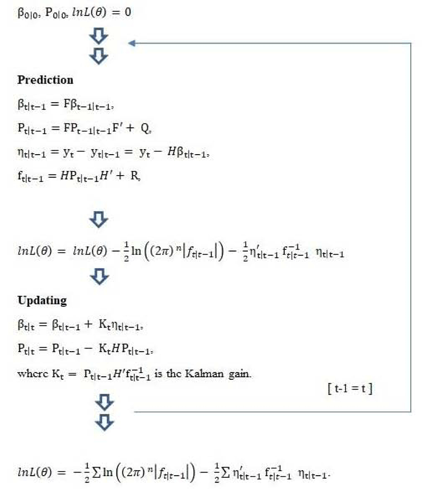
Assuming that H is available at the beginning of time t and a new observation of yt is made at the end of time t, the Kalman filter consists of the following two steps:
Given the system’s dynamics as expressed in Equations 1) and 2), the unobserved variable βt can be predicted by using the information up to the last period. This prediction yields βt|t−1, based on which we can predict yt, which yields yt|t−1. This process includes two uncertainties: The first is derived from the nature of the unobserved variable, as this variable cannot be directly observed. The second uncertainty is from the disturbance term in the measurement equation.
As the observed variable yt is realized, new information becomes available; specifically, the prediction error can be calculated from the realization of yt, and this can be used for a more accurate inference of βt. This updating step uses the so-called “Kalman gain,” which is the weight assigned to the new information about βt contained in the prediction error. However, βt|t (the estimate of βt) will be used as an input for the prediction in the next period.
The first model of this paper is a common stochastic trend model as follows:
In this model, y is the freight rate of considered dry bulk shipping markets. lnyi,t is influenced by the unobserved non-stationary common stochastic trend xt. This trend is assumed to be a random walk process without drift. The influence degree of estimated common stochastic trend on each variable is the coefficient γi, which is the measure for synchronicity. The idiosyncrasy is measured by . In particular, this common stochastic trend model decomposes the non-stationary (i.e., log-level) data into 1) non-stationary common permanent component (γi × xt) and 2) stationary transitory idiosyncratic component (ei,t). These equations can be represented by the following state-space model:
[Measurement Equation]
[Transition (or State) Equation]
The second model is a dynamic factor model as follows:
In this model, Δlnyi,t is the difference of logarithmic values of the freight rates, which is influenced by the unobserved stationary factor ct. This common factor is assumed to be an autoregressive process of order 1 whose parameter is ø. The influence degree of estimated common dynamic factor on each variable is the coefficient αi. which is the measure for synchronicity. The idiosyncrasy is measured by . In particular, this dynamic factor model decomposes the stationary (log-differenced) data into 1) stationary common component (αi × ct) and 2) stationary idiosyncratic component (ei,t). These equations can be represented by the following state-space model:
[Measurement Equation]
[Transition (or State) Equation]
The third model is an unobserved component model as follows:
In this model, lnyi,t is influenced by the unobserved non-stationary (permanent) stochastic trend xt and stationary (transitory) factor ct. The permanent trend is assumed to be a random walk process without drift and the stationary factor to be an autoregressive process of order 1. The influence degree of estimated common stochastic trend and dynamic factor on each variable are the coefficients γi and αi which are the measures for synchronicity, respectively. The idiosyncrasy is measured by . In particular, this unobserved component model decomposes the non-stationary (i.e., log-level) data into 1) non-stationary common permanent component (γi × xt) and 2) stationary common transitory component (αi × ct) and 3) stationary idiosyncratic component (ei,t). These equations can be represented by the following state-space model:
[Measurement Equation]
[Transition (or State) Equation]
4. Empirical Results and Discussions
This study uses the dataset consisting of the daily freight rates of Capesize and Panamax markets. In particular, as of 2021, one of the representative freight indicators for Capesize (18,000 DWT) is the 5TC average of the five routes for BCI (Baltic Capesize Index) produced by Baltic Exchange and for Panamax (82,000 DWT) is the 5TC average for BPI (Baltic Panamax Index). These data are all spot rates representing the current price for transporting dry bulk cargoes. The sample period ranges from 11th November 2017 to 20th May 2021. So, the number of observations is 885.
| - | Capesize | Panamax |
|---|---|---|
| Definition of variable | Average of the 5 T/C Routes for BCI | Average of the 5 T/C Routes for BPI-82 |
| Sample period | 11th November 2017 to 20th May 2021 | |
| Number of observations | 885 | |
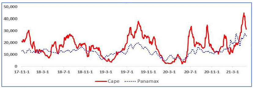
Figure 2 shows the movements of the Capesize 5TC and Panamax 5TC averages. As seen in this figure, there is some high correlations. The correlation is 0.68 in the level case and 0.30 in the log-difference case (Table 3). In addition, the determination coefficient (R2) of the regression from Panamax variable on Capesize variable is 0.88, which means that the two variables are highly correlated.
| - | Capesize | Panamax | |
|---|---|---|---|
| Level | Mean | 16,960 | 12,740 |
| Standard deviation | 8,544 | 4,174 | |
| Correlation | 0.68 | ||
| Log-differenced | Mean | 0.0004 | 0.0008 |
| Standard deviation | 0.0651 | 0.0250 | |
| Correlation | 0.30 | ||
All the values of original data are transformed into natural logarithms. Table 4 shows the unit root test results for checking the stationarity of the variables. For the log-level data, the null hypothesis is that a unit root exists in the case without a constant or trend. If it cannot be rejected at some significance level, then this means that the log-level variables are likely to be non-stationary. This non-stationarity enables us to adopt the stochastic permanent trend model. In addition, for the log-differenced data, the null hypothesis of the existence of unit root in the case without a constant or trend can be rejected at 1% significance level. This means that log-differencing the non-stationary variables makes them stationary. Therefore, this paper uses these stationary variables in the dynamic factor model.
| Capesize | Log-level | t-value | −0.045 |
| p-value | 0.667 | ||
| Log-differenced | t-value | −14.742 | |
| p-value | 0.000*** | ||
| Panamax | Log-level | t-value | 0.318 |
| p-value | 0.777 | ||
| Log-differenced | t-value | −10.441 | |
| p-value | 0.000*** |
2) The t-statistic refers to the Augmented Dickey-Fuller test statistic. Refer to Dickey and Fuller (1979, 1981).
4) The p-value implies MacKinnon’s (1996) one-sided p-value.
In order to apply the “common” stochastic trend model, there should be a cointegration relationship between the variables, the existence of which implies there is a common non-stationary stochastic trend. Table 5 shows that there is a cointegration relationship as predicted by the aforementioned structural characteristics of Capesize and Panamax freight markets. Its p-value is small enough to infer that there would be a cointegration relationship.
| - | Trace statistic | p-value |
|---|---|---|
| Number of cointegration Relationship: none | 22.053 | 0.028** |
| Number of cointegration Relationship: at most 1 | 4.965 | 0.287 |
| Cointegrating vector [1 βc] such that | [1 -1.826 7.603] | |
For the explanation of the trace statistic, refer to Johansen (1995).
The p-value means MacKinnon, Haug and Michelis (1999) one-sided p-value.
Table 6 shows the estimation result of common stochastic trend model. For the normalization of model, the variance of the shocks in the state equation is set to be 0.01. Similar to Ko (2010b, p.397), the influence coefficients are statistically significant. It is notable that the variance of idiosyncratic component in Capesize market () is very close to zero, which means that the unobserved common stochastic trend is estimated as close to the dynamics of Capesize variable. However, the two synchronicities of Capesize and Panamax (γc and γp) are very similar.
| - | Estimate | Standard error |
|---|---|---|
| γc | 0.659*** | 0.015 |
| γp | 0.645*** | 0.015 |
| 0.000 | - | |
| 0.203 | - | |
Table 7 shows the estimation result of dynamic factor model. For the normalization of model, the variance of the shocks in the state equation is set to be 0.0001. As the same as the common stochastic trend model, the two synchronicities of Capesize and Panamax (αc and αp) are very similar. However, the variance of idiosyncratic component in Panamax market () is very close to zero, which means that the unobserved dynamic factor is estimated as close to the dynamics of Panamax variable. In addition, it is notable that the persistence degree of the autoregressive process of unobserved dynamic factor, ø is 0.866, which is lower than in the unobserved component model of Table 8. However, the value of 0.866 means that the yesterday’s common factor influences today’s factor by this magnitude, 0.866.
| - | Estimate | Standard error |
|---|---|---|
| ø | 0.866*** | 0.014 |
| αc | 0.832*** | 0.006 |
| αp | 0.961*** | 0.005 |
| 0.004 | - | |
| 0.000 | - | |
Based on the results of Table 6 and Table 7, this paper constructs the unobserved component (permanent trends plus transitory cycles) model as a synthesizing model of common stochastic trend and dynamic factor models. That is, this paper recommends the use of the unobserved component (permanent trends plus transitory cycles) model rather than the separate uses of common stochastic trend model and dynamic factor model. Its estimation result is shown in Table 8. For the normalization of model, the variances of the shocks in the state equation and is set to be 0.0001, respectively. All the measures of synchronicities of common stochastic trend and dynamic factor (γc, γp, αc and αp) are very significant. In addition, it is notable that the persistence degree of the autoregressive process of stationary factor (ø) is 0.989, which is higher than simple dynamic factor model in Table 7. However, the variance of idiosyncratic component in Panamax market () is very close to zero.
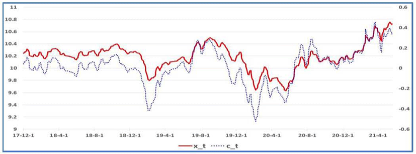
Based on the estimation result of Table 8, we can estimate the unobserved stochastic trend and cyclical factor. This paper calculates the so-called smoothed estimates of these two unobserved variables by using the full sample information and corresponding smoothing algorithm (see Kim and Nelson, pp.27-28), which is shown in Figure 3. As shown, the permanent trend (xt) and transitory factor (ct) move together.
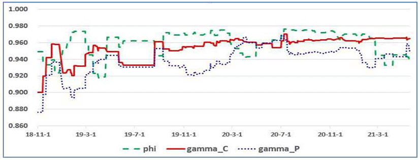
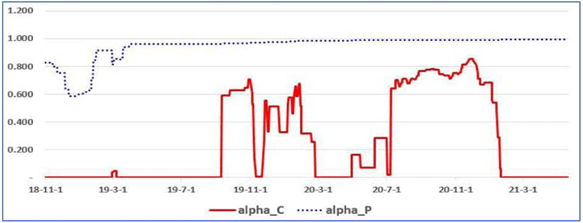
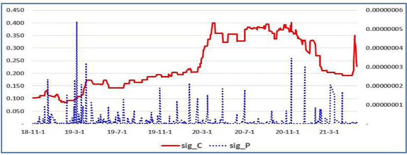
As discussed in Ko (2010a), the unobserved component model may suffer from parameter instability problem. Figure 4 to Figure 6 show the evolutions of the parameter estimates, rolling the estimation in the way, in which the sample consists of 12 months (one year) and thus depleting the first observation and adding the new last one. The choice of one year as the period of parameter rolling estimation is due to the fact that there is seasonality concern in more frequency cases, e.g., quarterly, monthly, etc. Overall, there seems to have been parameter instability. According to Stock and Watson (2016), in coping with this parameter instability, there could be two different approaches. First is to incorporate the break times in the considered model and another is to model time-varying parameters structure.
5. Conclusions
Based on the data of dry bulk shipping markets, this paper considers the three dynamic linear models such as common stochastic trend, dynamic factor, and unobserved component models by using state-space approach. All these dynamic linear models enable us to analyze the synchronicity and idiosyncrasy in the Capesize and Panamax freight markets in a coherent and efficient way. In particular, an unobserved component model, which incorporates the common stochastic trend and dynamic factor models, is proposed as a synthesizing approach. Using this unobserved component model, we can estimate the unobserved stochastic trend and dynamic factor via the Kalman filter and smoothing filter. This empirical investigation will help for the participants in dry bulk shipping markets to enhance the management efficiency of their revenues and market risks. In addition, this paper discusses the parameters instability problem by rolling the estimations whose sample consists of one year daily observations.
There remain three avenues for future research. First, based on the statistical significance of the dynamic linear models proposed in this paper (esp., unobserved component model), it will be possible to apply them to the more practical exercises, for example, forecasting the future rates. One of the causes of forecasting improvement would be the decomposition into the permanent and transitory components. More is there transitory elements, more successful is the forecasting. This is from the fact that by definition, the transitory components have a tendency to regress to the stationary expected value. That is, this tendency makes predictability. In contrast, the permanent components with random walk process, by its nature, are hard to predict. In other words, if we measure the transitory components, whether common or idiosyncratic, then by using this information, we can forecast the future direction of the considered variable conditioning on the recent information.
Second, the parameter instability shown in Figures 4-6 should be studied. This paper recommends that the first step is to model the variation of parameter values as an evolving process over time and, the second step is to incorporate break points if there is sudden change of parameter values. However, if it is recommended to model these breaks, state-space model with Markov switching regimes would be an excellent method, whose estimation can be done efficiently via the Kim filter (see Kim, 1994 and Kim and Kang, 2019).
Third, it would be promising to investigate more structural characteristics of dry bulk shipping markets based on the reduced-form analyses of this paper. If the above second future research about the structural breaks in parameter values would provide some acceptable estimates on the break timings, then the comparisons among the different regimes would enable us to more understand the relevant markets. This enhancement of knowledge on the market dynamics will help the participants in dry bulk shipping markets to manage their revenues, cost, or market risks.
As a final remark, the recommended model for the dry bulk shipping freight rate movements by using some synthesizing unobserved component model with time-varying coefficients can be a good indicator for the decision making on the chartering strategies of shipowners or charterers. Furthermore, more investigation of structural characteristics of dry bulk shipping markets based on this model could yield fruitful information for the market participants and relevant policy makers.


