Mega Vessels – Mega Error?

1. Background

Ultra Large Container Ships (ULCS) with more than 12,000 TEU capacity have become the work-horses of deep sea container shipping. The reason for the growth to currently up to 24,000 TEU, which many industry experts have not believed to be possible some years ago, is the intention to intensify the use of the economies of scale (EoS) in order to further reduce the costs per carried TEU.

Competition in container shipping is mainly by price. Hence container carriers are naturally aiming at being a cost leader. The utilisation of the EoS effects is a powerful tool in this respect as shipbuilding and fuel prices as well as operational cost, i.e., mainly for crewing, are more or less the same for all carriers. It has already been shown that these three types of specific costs per TEU follow asymptotic curves, the course of which becomes flatter with increasing ship sizes (Malchow, 2014; 2015; 2017). The cost advantage per TEU therefore decreases with the size of the ship, while the carriers are facing more operational challenges in terms of nautical restrictions, higher average risks and damages as well as longer port stays which certainly influences the economics as well. However, this is obviously being widely ignored as the increase in ship sizes continues.

Among maritime economists it is meanwhile widely recognised that the ocean carriers are reducing their costs by introducing ever bigger ships on costs of the other players within the intermodal transport chain: if all the public and private investments were taken into account that had to be made in the ports and for hinterland transport in order to cope with the dimensions of the giant ships and the extreme peak loads they are causing, it would have to be concluded that there is no general economic benefit left from the overall perspective (Malchow, 2018; Merk, 2015). In view of the current considerations to go even beyond the current maximum of approx. 24,000 TEU and the fact that the Suez Canal Authority has already decided to further expand the canal, which would allow this jump, it can be taken for granted that even in what has become a very consolidated carrier environment there will be always a shipping line that would blindly follow the path of supposedly limitless growth without deep thinking. Experience has shown that the other market participants would then feel forced to follow in order not to supposedly fall behind in the competition for the lowest slot costs. Hence, another round of the growth spiral would have been started. Such mechanism is still supported by recent studies which claim to have identified EoS effects for the operation of ships of 24,000 TEU and beyond (Alphaliner, 2021; Ge et al., 2019; Rasewsky, 2021). Even hypothetical ship sizes of up to 50,000 TEU are said to provide still economic benefits to their operators (Saase, 2018; Saxon and Stone, 2017).

It is therefore to be examined to what extent the use of these ships still makes sense also from the shipping line’s perspective. The focus is on the effects of the inevitably longer port stay of the ULCS, i.e., its dependence from the ship size and its consequences for ship operation. In order to be able to make generally valid statements, which are independent from the specifics of individual ships and ports, and to avoid highly complex individual calculations, generally valid proportionalities shall mainly be applied.

2. Calculation

Any round voyage is basically consisting of time shares for navigating and port stay, which in turn can be subdivided into the time for coastal navigation (normally connected with speed restrictions) and the time at sea as well as into the time for pure container handling and various waiting times in port:

Time for coastal navigation (incl. canals) as well as unproductive waiting times in and off the ports (e.g., for shifting of gantry cranes, hoisting/lowering their jib, waiting for tide, pilot or start of shift as well as interruptions of work by labour breaks or weather and of course congestion of ports itself etc.) are considered to be constant in total and independent from ship size and its speed. They are summarised under t_{coastal+waiting}. Nowadays a typical round voyage between Northern Europe and the Far East lasts 12 weeks with the following time proportions:¹

For the calculation of the required accumulated pure container handling time across all ports, it is assumed that the full (nominal) container capacity of a ship CC [TEU] is being loaded and discharged in each trade direction (wayport cargo and restowage of containers not being considered). With this approach the actual number of ports among the containers are distributed is irrelevant. The respective times in their coastal waters and for waiting within or off the ports are already included in t_{coastal+waiting}.

The accumulated pure container handling time across all ports t_{container handling} is generally determined by the number of containers to be handled, i.e., the quadruple full container capacity of the ship 4CC (2×loading, 2×discharging), multiplied by the average utilisation rate of the ship UR[%] which is to be divided by the prevailing TEU factor TF[TEU/Ctr], the average handling rate of the gantry cranes in the particular trade HR [Ctr/hr] and the number of cranes which can be placed alongside the ship n_C:

The handling rate of the gantry cranes depends on their handling speed (trolley and hoisting speed), their standard (e.g., 2-trolley operation, 4-TEU spreader), the skills of the crane driver and the path length of every single container load cycle. The properties of the crane equipment and the resulting speed vary from port to port and do not depend on the ship size (assumption: all ships can be served with the same cranes). Hence they do not need to be further considered as they fall out as a constant factor. Only the path each container has to cover depends very much on the ship size.

In order to determine the average path length the main frame cross- section of several vessels sizes from 1,100 TEU up to 32,000 TEU (projected) are examined with the help of a simple box grid (Figure 1). Sizes above 24,000 TEU are still hypothetical but respective design studies do already exist (Alphaliner, 2021; Rasewsky, 2021). Also geometric design variants within a size class are taken into account (e.g., less beam but instead more layers on the hatch covers or in the hold). The individual path from each stowage position is determined by simply counting the boxes that each container has to cover to a common position on the pier that is identical for all containers of all ship sizes. Subsequently for each of the cross-sections the value for the average distance all containers have to cover is determined while the unit of the distance is not relevant. It could be kept as ‘boxes’ as an equivalent.

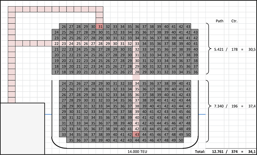
In reality vertical and horizontal motions are combined which reduces the actual length of the path. These shortcuts are assumed to be independent from the ship size. The differences between the individual trajectory curves would remain. Hence, the shortcuts can be neglected and the results from the ‘angular’ trajectories remain valid. Two common premises which shall be valid for all cross-sections are set in order to compare on the same basis (Figure 1):

Even if these premises were not fully in line with the reality their common application would ensure meaningful results. The absolute values of the premises are only of secondary importance as long as they are generally applied.

The examined ship sizes with their various cross-sections result in an exponential function of high regression quality for the average length of the container handling path (number of ‘boxes’) (Figure 2). The exponent is positive but significantly smaller than ‘1’, i.e., the average path length of the containers grows with the ship size but less than proportionally. Thus, the achievable handling rate HR of the cranes decreases with increasing ship size – also less than proportionally (regardless of the actual performance of the cranes):

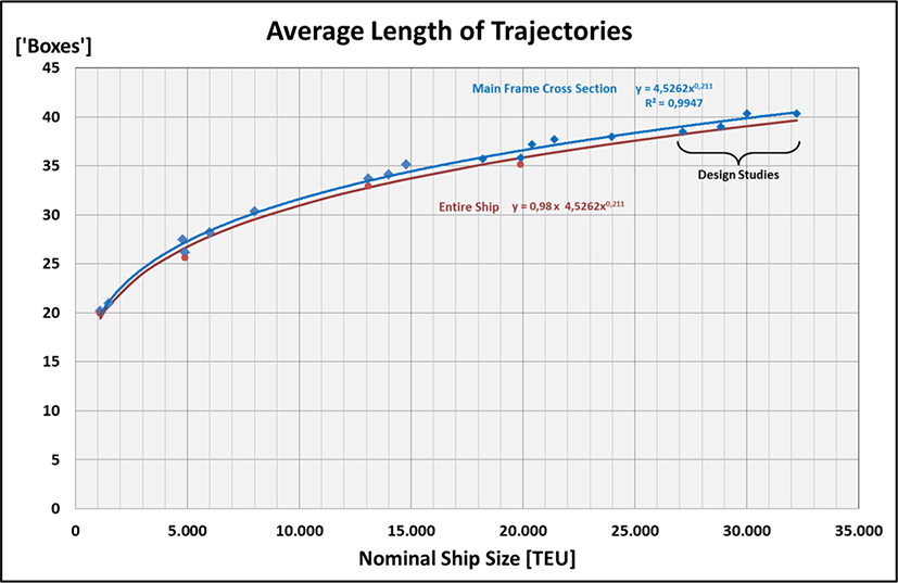
Equation (5) coincides very well with the statement of Lai (2015) as a practitioner (MD, Modern Terminals Ltd., Hong Kong), who already reported at that time that the average path of the containers during ship-to-shore handling has been extended by approx. 50% when comparing the so-called ‘Triple-E’ class vessels of Maersk (18,300 TEU) with Panamax vessels of approx. 4,500 TEU.

However, the main frame cross-section is not representative for the entire vessel. Towards the ship’s ends the number of containers, in particular within the holds, is getting less. Hence, for 4 exemplary ship sizes (1,100 TEU, 4,900 TEU, 13,100 TEU, 19,900 TEU) the ‘path lengths’ in terms of crossed ‘boxes’ are determined for each individual container. Subsequently the average value for the total ship is calculated. Result: for all of the examined ships it turns out that the average value for the entire ship is virtually constantly 98% of the average value for its main frame cross-section. Hence, general validity is assumed. Since this percentage is to be regarded as a constant factor, the general validity of the proportionality according to equation (5) does not suffer.

The number of gantry cranes which can be placed alongside a ship is by nature in proportion to the ship’s length even though it is not a continuous relation: the ship’s length has to be increased by at least 2×40 ft bays to place one further crane. Furthermore a minimum gap between the cranes has to be kept for safety and operational reasons. In reality ship sizes do not increase continuously either. However, in order to discover a general context all calculations are based on the (unrealistic) assumption of continuous functions.

For the length between perpendiculars LPP of container ships Abramowski et al. (2018) have determined following logarithmic regression equation for ships of CC < 20,000 TEU (R² = 0.978) whereas the data supply for ships of CC > 14,000 TEU was rather poor with only 7 vessels:

The length between perpendiculars LPP is increased by 5% (average from author’s data pool) to get the length over all LOA (green line in Figure 3). However, with respect to this particular data pool equation (6) results into too little values for small ships whereas for ULCSs the values are too high.

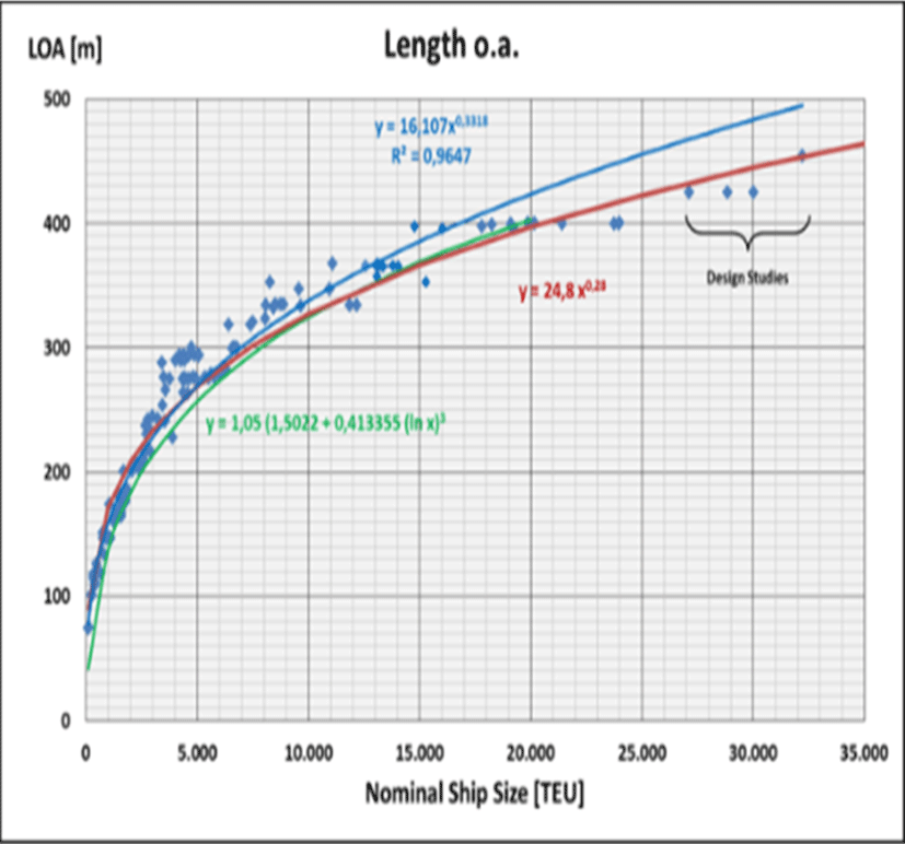
The cubic law of geometry states that the dimensions of a cuboid grow with the 3^rd root of its volume (L, B, H ~ V^1/3). The high regression quality of a corresponding analysis of a large number of container ships confirms in principle this law with respect to the ratio of the ship’s container capacity CC to its length over all LOA (blue line in Figure 3). However, it can be derived from the diagram that the high regression quality essentially refers to the high number of smaller ships in the author’s data pool. For the larger ships of interest, of which significantly less data are available, the regression equation clearly results in ship lengths that are too long. For the actual ULCSs (incl. design studies of up to 32,000 TEU) (Alphaliner, 2021; Rasewsky, 2021) the following exponential equation describes the relation between the length over all LOA and the container capacity CC apparently much better (red line in Figure 3):

Equation (7) is also very much in line with the findings of Park and Suh (2019), who have ascertained for container ships of CC > 7,000 TEU: L = 25.08 CC^0.28. Accordingly, the number of deployable cranes n_C versus the container capacity CC grows generally even less than according to the cubic law (whereby the actual absolute number of cranes that can be placed is irrelevant in this consideration):

When equation (5) and equation (8) are plugged into equation (4) it follows that the accumulated pure container handling time t_{container handling} basically increases proportionally to the container capacity CC:

The practical proportionality results from the fact that the exponents for determining the handling rate HR (equation (5)) and for the number of deployable cranes n_C (equation (8)) add up to almost zero. I.e., the generally longer container trajectory of bigger ships and the number of gantry cranes which do not increase proportionally to the ship size effect that the accumulated pure handling time of the containers is virtually proportional to the ship’s container capacity CC (equation (10)). The average utilization of the ship UR, the speed of the individual crane HR, the number of employed cranes n_C and the actual TEU factor TF can be neglected as they are constant factors when just proportionality is being considered. If the number of cranes cannot actually be increased according to the ship’s length (e.g., as not enough are available) t_{container handling} grows even more than proportionally to CC.

If the duration of a round voyage is to be kept constant while the time for container handling increases, in order to keep the sailing frequency (e.g., for fixed day sailings) and/or not to increase the number of vessels employed, the time at sea must be consequently reduced by a higher ship speed:

For the established proportionality between the accumulated pure container handling time t_{container handling} and the container capacity of the ship CC as per equation (10) the proportionality factor k_i [days/TEU] as so-called ‘handling factor’ is being introduced (equation (12)). This factor describes the average handling productivity within a particular liner service as the result of the technical performance of the handling equipment and soft factors such as the qualification of staff or the labor shift scheme. k_i is defined to be independent from the ship size but for reference it should be indicated at which size it has been originally measured:²

The time at sea t_sea is given by the fixed distance s_sea divided by the average speed of the ship v_Ø. The given duration of the round voyage t_{round voyage} and the fixed deductions t_{coastal+waiting} which are independent from the ship size and its speed are summarised under t_{round voyage′}:

After the formation of the reciprocal following proportionality can be established (as the distance s_sea remains constant by nature):

With the help of the so-called ‘Admirality Formula’ which is used in preliminary ship design the propulsion power P can be estimated when the displacement Δ [t], the speed v_Ø [knots] and also the Admirality Coefficient C_Admiral is known. The fuel consumption ṁ_fuel [tons/day] is directly proportional to the propulsion power (in a certain bandwidth):

From the available container ship data an almost linear equation of high regression quality for the relation between container capacity and displacement (scantling) can be derived, i.e., the exponent of the exponential equation has a value of almost ‘1’ (Figure 4). The high quality of the almost linear regression equation is again based on numerous smaller ships. For ULCS it provides apparently too high values (for projected ships of CC > 24,000 TEU no corresponding values for Δ are anyhow available yet). For ships of CC < 20,000 TEUAbramowski et al. (2018) have found a logarithmic regression equation (R² = 0.994) whereas with only 7 ships of CC > 14,000 TEU the related data base was rather poor:

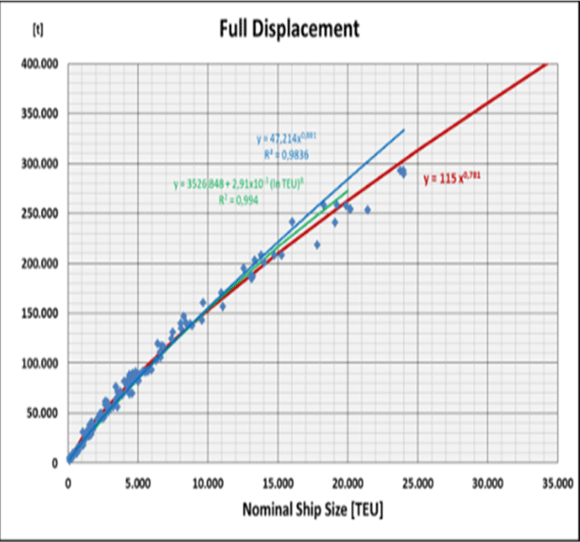
Apparently also this equation results into too high values for big ships (green line in Figure 4). Hence, this equation needs also to be adjusted. Following exponential equation reflects the full range of ship sizes much better (red line in Figure 4):

According to equation (15) the fuel consumption ṁ_fuel [tons/day] for propulsion is generally proportional to Δ^2/3 as well as to v_س(as C_Admiral remains practically constant for the category of ULCS it can be disregarded when considering proportionality)³:

Expanding equation (18) with t_sea and CC^-1 results into the proportional dependence of the specific fuel mass per TEU (for propulsion) needed for the entire round voyage (equation (20)):

For Δ, v_Ø and t_sea the equations (17), (14), and (13) are plugged into equation (20) which is subsequently reshaped:

Hence, a proportional dependence of the required specific fuel quantity per TEU m_fuel/CC (over the entire round voyage) from a term just containing the ship size CC, the duration of the round voyage (minus the fixed time shares) t_{round voyage′} and the container handling factor k_i is found! The same applies for the specific CO₂ emissions per TEU m_CO2/CC as they are proportional to the respective fuel quantity just by matter of chemistry:

For t_{round voyage′} typical values from real liner services can be inserted, e.g., for a typical Northern Europe – Far East round voyage of 12 weeks (equation (3)):

The container handling factor k_i can be calibrated for a particular liner service with the help of the actual pure handling time accumulated over the entire round voyage t_{container handling} which is to be divided by the nominal container capacity CC of the respective ship (here: 13,000 TEU):¹

The term (t_{round voyage′} − k_i CC)⁻² in equation (22) is equivalent to the reciprocal square of the time at sea t_sea. The shorter it becomes (to maintain the duration of the round voyage with longer container handling time in port) the more fuel is needed in the course of the round voyage (with quadratic effect). This is counteracted by the EoS effect – but only with the factor CC^−0.479. This exponential function results into an asymptotical curve, i.e., the EoS effect becomes smaller with increasing ship size. The term (t_{round voyage′} −k_{i CC})⁻² reflects the basic operational parameters of a particular liner service. Beside CC only t_{round voyage′} and k_i are needed as variables to investigate the dependence of the specific fuel demand per TEU from the ship size.

The entire term CC^-0.479 (t_{round voyage′} –k_i CC)^–2 of equation (22) has no meaningful unit but is proportional to the required quantity of fuel per TEU during the round voyage or emitted CO₂ per TEU respectively! It does not state the required fuel quantity itself! The actually needed fuel quantity is just proportional to this newly created ‘Fuel/TEU Indicator’. Hence, it is interesting to see whether the indicator has a minimum and in the affirmative whether it is within the range of already existing or to be expected ship sizes.

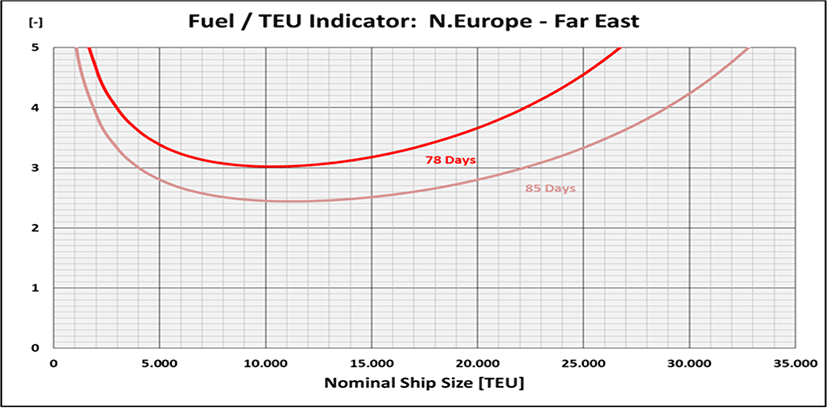
It reveals that for a typical Northern Europe – Far East round voyage with t_{round voyage′} = 78 days and k_13,000 = 1.462 × 10^–3days/TEU the Fuel/TEU Indicator has indeed a minimum at CC ≈ 10,300 TEU (read from Figure 5)!

3. Results

For any liner service the optimal ship size with regard to the minimum quantity of required fuel per TEU and per round voyage which results also into minimum CO₂ emissions per TEU can be easily estimated by applying equation (34). For a typical Northern Europe – Far East round voyage of 12 weeks (see above) the exactly calculated optimal ship size with regard to the lowest Fuel/TEU Indicator would be:

According to equation (34) the ship size at which the Fuel/TEU Indicator reaches its minimum is proportional to t_{round voyage′} and inversely proportional to k_i. With other words: the optimum size increases proportionally with the duration of the round voyage (minus the fixed time shares for coastal navigation and waiting times in port) and inversely proportional with the average pure handling time per TEU over the total ship capacity. This in turn means that the longer the variable times of the round voyage (for container handling and sea voyage) and/or the smaller the handling factor the bigger is the ship size where the Fuel/TEU Indicator finds its minimum:

E.g., if the duration of the round voyage was extended by slow steaming by 9% to 13 weeks, i.e., t_{round_voyage′} = t_{round voyge} – t_{coastal+waiting} = 91 days - 6 days = 85 days (consequently requiring a 13^th ship when the sailing frequency and the transport capacity is to be maintained), the fuel demand per TEU would be naturally significantly less and the calculated minimum of the Fuel/TEU Indicator would also increase by 9% to CC_{fuel min} = 11,233 TEU (Figure 5). CC_{fuel min} would be correspondingly lower if the duration of the round voyage was shortened.

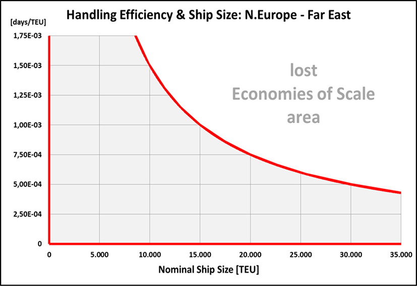
Beside the handling factor of k_13,000 = 1.462 × 10^–3days/TEU which is determined with a ship size of CC = 13,000 TEU further curves of the Fuel/TEU Indicator for handling factors of k_13,000 = 0.75… 1.75 × 10^–3days/TEU are investigated while applying equation (34) (Figure 6): it is quite obvious that increasing the handling efficiency results into a lower curve of the Fuel/TEU Indicator as the average speed at sea can be reduced. Furthermore the ‘optimum’ ship size is moving towards bigger ships and the increase after passing the minimum is the flatter the higher the handling efficiency is. The dashed line in Figure 6 connects the minimum points of each curve. Hence, with regard to the specific fuel quantity and/or the CO₂ emissions per TEU combinations of ship size and handling factor above that line do obviously not make any sense! For the investigated North Europe – Far East trade Figure 7 illustrates the resulting ‘no go area’ for combinations of ship size CC and handling factor k_13,000 above the border line curve where no EoS effect with regard to the fuel quantity and/or the CO₂ emissions per TEU can be expected any more.

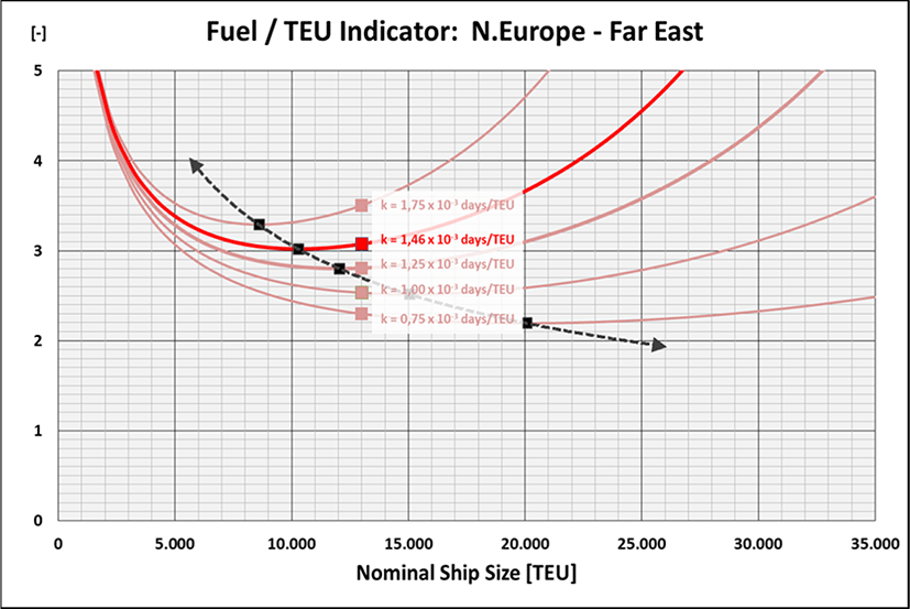
Amazing realization out of Figure 6: instead of operating 20,000 TEU ships on a Northern Europe – Far East liner service with a handling factor of k_13,000 = 1.462 × 10^–3days/TEU twice the number of 10,000 TEU ships navigating at a lower speed were more efficient with regard to the consumed fuel and CO₂ emissions per TEU. Incidentally it should be noted that such configuration would also increase the service quality in terms of a doubled sailing frequency. Obviously only from a handling factor of k_13,000 = 0.75 × 10^–3days/TEU ≈ 1 min/TEU and less ships of CC = 20,000 TEU start to make sense. Provided no tandem or 4-TEU spreaders are used and a TEU factor of TF = 1.6 TEU/Ctr applies such value for k_13,000 would correspond to an average total ship handling rate of:

If in all ports an average number of e.g., 6 gantry cranes served the ship, it would correspond to an average handling rate of HR = 25 moves/hr per crane which is not unrealistic.

A container terminal in Shanghai has recently reported on the biggest ever handled container volume with one ship: within 62 hours 25,775 TEU were handled with a ship of about 23,000 TEU size. Up to 11 gantry cranes were said to be intermittently employed (World Cargo News, 2021). Provided a TEU factor of TF = 1.6 TEU/Ctr this corresponds to 260 moves/hr. Assuming that only 8 to 10 cranes were employed in average this corresponds to a handling rate per crane of HR = 32.5… 26.0 moves/hr.

However, at assumed present average handling efficiencies the common ship sizes in the Northern Europe – Far East trade of today are therefore operating well above the optimal ship size derived from general physical and geometric relations, where the quantity of fuel and thus also the CO₂ emissions per TEU are at a minimum! At an assumed handling factor of k_13,000 = 1.462 × 10^–3days/TEU the Fuel/TEU Indicator of the currently largest ships of around 24,000 TEU is in the same range as of ships smaller than 5,000 TEU (when navigating at slower speed)!

4. Overall View

Beside the fuel cost per TEU two further specific cost items are of major importance for the ship operator:

Both types of costs benefit from continuous EoS effects without opposing effects occurring. However, the corresponding curves become flatter in the course of increasing ship sizes. The specific light weight of the ship per TEU (for capital costs) and the manning level per TEU (for operating costs) have been already introduced and derived as suitable and ‘neutral’ indicators for both types of costs (Malchow, 2015). The advantage of this approach is that these sizes are not influenced and possibly hidden by price, interest level or exchange rate parities resulting from changing market conditions. They are unambiguous values that cannot be falsified, whereby the data on the empty ship weight are unfortunately not easy to obtain. The absolute number of manning is not even required as only the reciprocal relationship is relevant, which means that the relevant costs per TEU are e.g., halved, when the ship size doubles.

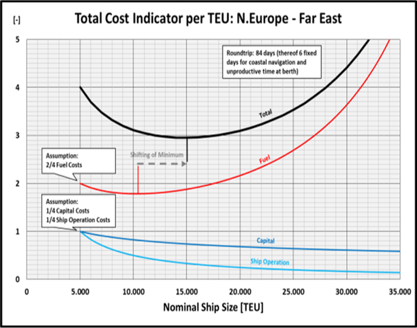
All three indicators can be combined to a Total Cost Indicator, whereby it is initially assumed that the three types of costs are each weighted with ⅓ at a starting point, which appears to be not unrealistic. This point is arbitrarily set at a ship size of 5,000 TEU (slightly larger than the Panamax ships usually operated at earlier days in the Northern Europe – Far East trade) and standardised in such a way that each cost type has a starting value of ‘1’ (without any unit). Then the three curves are added (Figure 8).

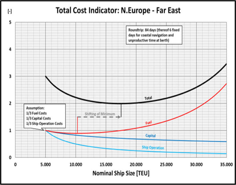
For a typical Northern Europe - Far East service, it can be derived from the diagram that under the above mentioned premises for the three types of specific costs, and thus also in the overall view, an initially very strong degression of costs results from the initially dominating EoS effect up to a ship size of about 12,000 TEU. Above approx. 17,500 TEU the influence of the Fuel/TEU Indicator, which already rises again from 10,308 TEU onwards (see above), is greater than the ever weaker decrease in capital and ship operating costs. Hence, in the overall view also the Total Cost Indicator rises from there.

Should the fuel costs at the starting point make up actually a larger proportion of the total costs per TEU than the estimated ⅓, e.g., by a doubled fuel price which consequently would increase the weighting of the fuel costs from ⅓ to ½ and let the Total Cost Indicator starts at ‘4’, the Total Cost Indicator would already reach its minimum at approx. 15,000 TEU instead of 17,500 TEU (Figure 9). The reverse applies accordingly. In reality the share of fuel costs can be indeed expected at somewhere between ⅓ and ½ (Garrido et al., 2020).

5. Other Trades

Two other important trades in global container shipping have been investigated as well as per Table 1. Across the Pacific smaller ships are employed and the duration of the round voyage is significantly shorter (t_{round voyage′} = 38 days) while the container handling productivity is higher (k_8,500 = 1.2 min/TEU). The course of the curves for the indicators for capital and ship operating costs is by nature independent from the trading area. However, the minimum of the Fuel/TEU Indicator is already reached at around 9,000 TEU (Figure 10).

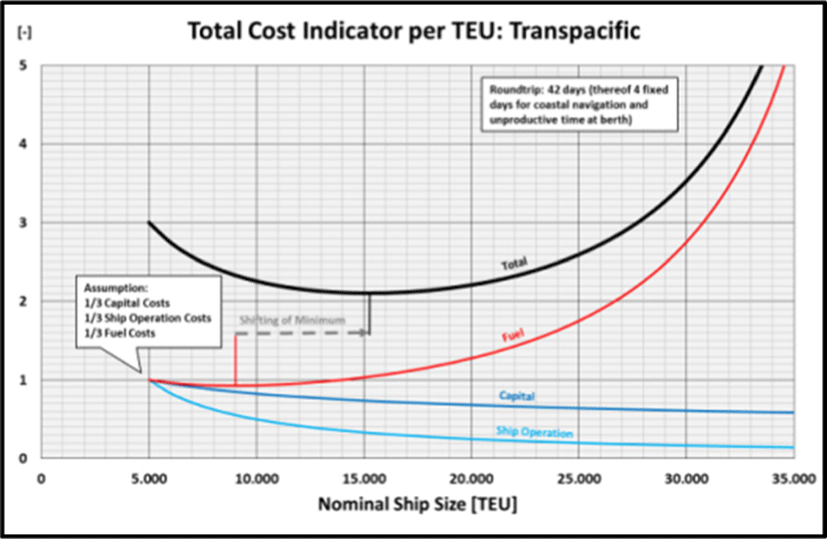
Consequently, also the Total Cost Indicator finds its minimum at a smaller ship size. Due to the shorter duration of the round voyage less time is available to compensate for longer port stays, i.e., the increase in speed and thus the resulting quantity of fuel per TEU has a greater impact (with a quadratic effect).

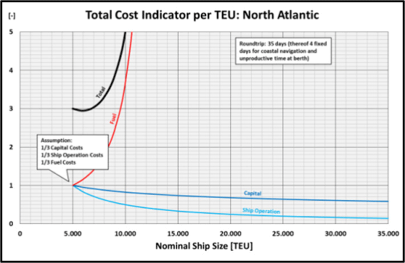
On the North Atlantic the ships are even smaller and the duration of the round voyage is even shorter while the overall container handling is significantly less productive (k_4,500 = 3.2 min/TEU). Hence, the situation is even more extreme (Figure 11): the minimum of the Fuel/TEU Indicator is still below the starting point at 5,000 TEU, which results into the minimum of the Total Cost Indicator being located only slightly above the starting point at about 6,000 TEU. Due to the relatively short time at sea, the required acceleration is extreme to compensate longer handling times. The Fuel/TEU Indicator rises so steeply that the technical feasibility at all is in question. The enormous propulsion power which would result from the required speed, would lead to space requirements for the engine plant which would require a completely different ship!

6. Findings

Referring to the initial questioning of the alleged endless EoS effects in container shipping following conclusions can be drawn:

7. Discussion

The present study is based on the interaction of fundamental geometrical and physical relationships, from which generally valid proportionalities are derived. By using non-monetary values as the basis for a corresponding cost trend, ‘neutral’ expenses can be derived that are free of ‘commercial coincidences’ such as market prices, currency parities, volume discounts, negotiating skills or the level of interest rates.

The introduction of the dimensionless Fuel/TEU Indicator allows the required conclusions regarding the size-dependence of the fuel requirement per TEU without the need for complex calculations of the absolute consumption of various ships under varying circumstances and various assumptions.

The merger of the Fuel/TEU Indicator with the indicators for capital and ship operating costs via normalisation and (arbitrary but realistic) internal weighting to a dimensionless Total Cost Indicator allows for further cognitions of the relationship between ship sizes and overall economics.

The following simplifications have been made and should be assessed: